IBM Optimizations using Qiskit

Below is a brief tutorial on Superstaq optimizations for IBM Quantum superconducting qubit devices. For more information on IBM Quantum, visit their website here.

Imports and API Token

This example tutorial notebook uses qiskit-superstaq, our Superstaq client for Qiskit; you can try it out by running pip install qiskit-superstaq[examples]:

try:
    import qiskit
    import qiskit_superstaq as qss
except ImportError:
    print("Installing qiskit-superstaq...")
    %pip install --quiet 'qiskit-superstaq[examples]'
    print("Installed qiskit-superstaq.")
    print("You may need to restart the kernel to import newly installed packages.")
    import qiskit
    import qiskit_superstaq as qss

import numpy as np

To interface Superstaq via Qiskit, we must first instantiate a provider in qiskit-superstaq with SuperstaqProvider(). We then supply a Superstaq API token (or key) by either providing the API token as an argument of qss.SuperstaqProvider() or by setting it as an environment variable (see more details here)

# Provide your Superstaq API key using the "api_key" argument
provider = qss.SuperstaqProvider()

Single Circuit Compilation

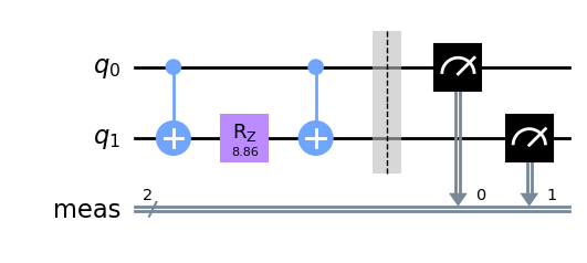
Let us start by creating an example Qiskit circuit that we will then compile and optimize for the 127-qubit IBM Quantum brisbane processor.

# Create a two-qubit qiskit circuit
theta = np.random.uniform(0, 4 * np.pi)
circuit = qiskit.QuantumCircuit(2)
circuit.cx(0, 1)
circuit.rz(theta, 1)
circuit.cx(0, 1)
circuit.measure_all()

# Draw circuit for visualization
circuit.draw(output="mpl")

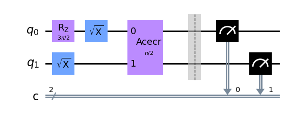
We will now compile the above circuit to IBM’s brisbane processor and visualize the differences by drawing the compiled circuit.

# Compile with ibmq compile
compiler_output = provider.ibmq_compile(circuit, target="ibmq_brisbane_qpu")

# Call circuit from the compiler output to get the corresponding output circuit
output_circuit = compiler_output.circuit

# Visualize the compiled circuit
output_circuit.draw("mpl", idle_wires=False)

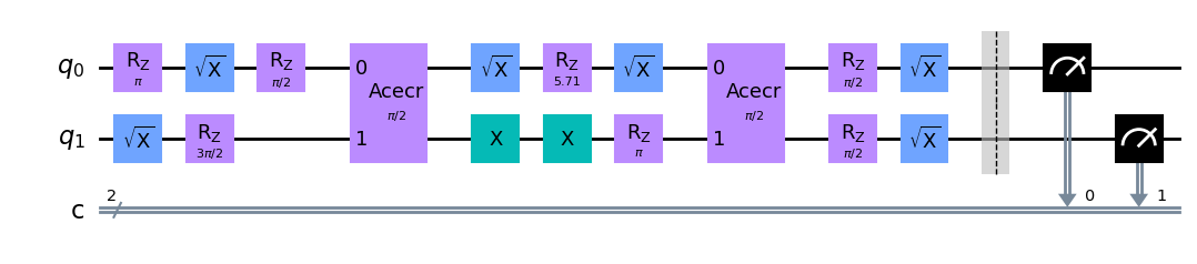
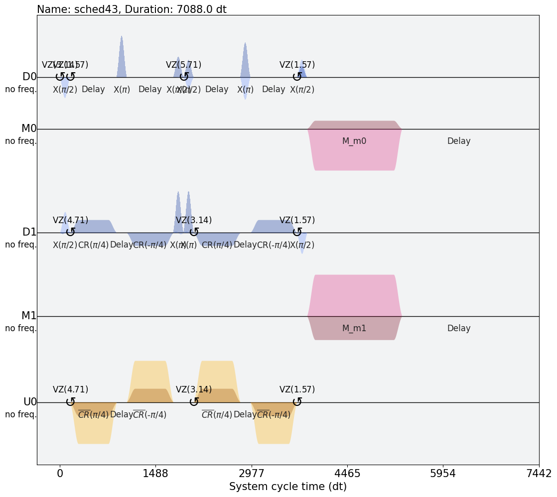
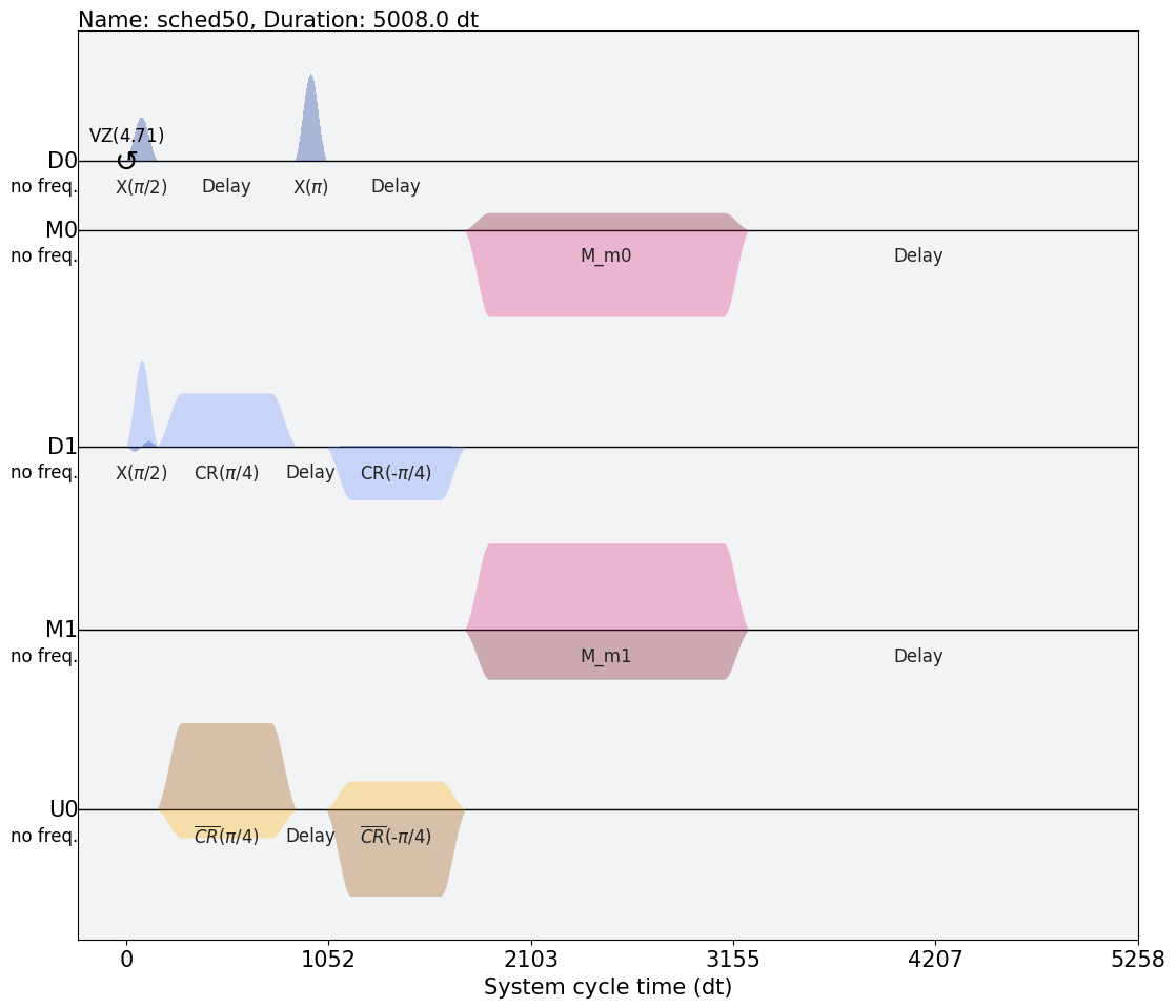
The resulting output is now a circuit compiled to brisbane’s native operations. With Superstaq compilation, you can also get the corresponding Qiskit Pulse schedule (see Qiskit Pulse documentation and original paper) for the compiled circuit by running the following:

# Visualize the pulse schedule using Qiskit Pulse
compiler_output.pulse_sequence.draw()

Multiple Circuits Compilation

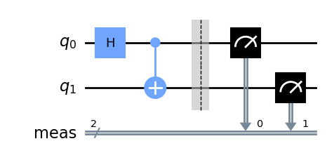
All the functionalities we have seen so far can also be used on a multiple-circuit input as well. To illustrate this, let us create a different example two-qubit circuit: a Bell-state circuit.

# Create second circuit
bell_circuit = qiskit.QuantumCircuit(2)
bell_circuit.h(0)
bell_circuit.cx(0, 1)
bell_circuit.measure_all()

# Draw second circuit for visualization
bell_circuit.draw("mpl")

By passing multiple circuits as a list to the ibmq_compile endpoint, we can compile all of them individually with a single call to the endpoint. This will return all the corresponding compiled circuits and Qiskit Pulse schedules back as a list, like so:

# Create list of circuits
circuit_list = [circuit, bell_circuit]

# Compile list of circuits
compiler_output_list = provider.ibmq_compile(circuit_list, "ibmq_brisbane_qpu")

# The list of compiled output circuits is stored in the `circuits` attribute instead of `circuit`. Likewise for
# pulse sequences.
output_circuits = compiler_output_list.circuits
output_pulse_sequences = compiler_output_list.pulse_sequences

# Visualize the first compiled circuit
print("Compiled circuit 1 \n")
output_circuits[0].draw("mpl", idle_wires=False)

Compiled circuit 1

# Visualize the pulse sequence for the first compiled circuit
output_pulse_sequences[0].draw()

# Visualize the second compiled circuit
print("Compiled circuit 2 \n")
output_circuits[1].draw("mpl", idle_wires=False)

Compiled circuit 2

# Visualize the pulse sequence for the second compiled circuit
output_pulse_sequences[1].draw()

Using Superstaq Simulator

Lastly, we will show (a) how to execute a circuit on a backend and (b) how to simulate circuit execution. Simulation is available to free trial users, and can be done by passing the "dry-run" method parameter when calling run() on the Superstaq provider.

# Get IBM Quantum backend from provider
backend = provider.get_backend("ibmq_brisbane_qpu")
job = backend.run(
    bell_circuit,
    shots=1000,
    method="dry-run",  # Specify "dry-run" as the method to run Superstaq simulation
)

# Get the counts from the measurement
print(job.result().get_counts())

{'00': 502, '11': 498}

Addendum: Compiling via Superstaq backend

You can also compile circuits via the compile method of the backend directly. This is identical to calling ibmq_compile on the provider, but more closely matches Qiskit syntax.

compiler_output = backend.compile(bell_circuit)
output_circuit = compiler_output.circuit
output_pulse_sequence = compiler_output.pulse_sequence

# Visualize the compiled circuit
output_circuit.draw("mpl", idle_wires=False)

# Visualize the pulse sequence
output_pulse_sequence.draw()